Category Archives: Astronomy

Imaging Comet 46P/Wirtanen

Sunday night, December 16th, was the evening of the closest approach of Comet 46P/Wirtanen. The comet was close enough and bright enough with an apparent magnitude between 4.0 and 4.5 that you could see it with the naked eye if you had good, dark skies. Thankfully, that’s just what I have living out in rural Missouri, and we also had crystal clear skies. The comet can be seen between the Pleiades Cluster and Taurus through Wednesday, but as the Moon’s phase transitions from 1st Quarter to Waxing Gibbous, dim objects in the sky will be harder and harder to see. Throughout this coming week, the best time to view the comet will actually be in the very early morning after moonset. You can check out more about where to find and when to view the comet at Sky and Telescope, https://www.skyandtelescope.com/astronomy-news/observing-news/comet-46p-wirtanen-and-moon/.

Comet 46P/Wirtanen passing between the Pleiades Cluster and Taurus.

The image below of Comet 46P/Wirtanen is the result of stacking 63 exposures each with a shutter speed of 20-seconds, ISO 6400, aperture f/8, and a focal length of 200 mm on a Nikon D500 through a Tamron 70-200mm f2.8 riding atop a Celestron 8″ SCT. The telescope was there just to provide the clock drive so that the camera moved with the stars’ diurnal motion. Each raw image file was corrected for dark current, bias current, and the response across the frame was normalized using a flat field image. I’ll write up a tutorial on how to collect these images and why they’re necessary later. The images were then aligned and stacked on the comet, which is why the stars appear as streaks. Since the comet is moving quite rapidly past us, its motion relative to the distant background stars is very noticeable, even in the short timespan of this image set.

An long exposure image of Comet 46P/Wirtanen tracking the comet’s motion rather than the stars’ motion.

You may have noticed the very green color to many of the images of Comet 46P/Wirtanen, including this one. The green color is not a image processing artifact, but is indicative of the comet’s composition. Most comets contain a enough cyanogen (CN) and diatomic carbon (C2). As a comet approaches the Sun and its surface warms, volatile materials such as cyanogen, water, and others begin to vaporize forming the comet’s coma and tail. When cyanogen and diatomic carbon interact with the Sun’s ultraviolet light and fluoresce to create the characteristic greenish glow of many comets.

Voyager II Is Outta Here!

Well, perhaps more precisely, the Voyager II spacecraft is now making its way through the heliopause region.  Unlike planetary magnetospheric boundaries, the boundary between the heliosphere and the local interstellar medium (LISM) has substantial thickness compared to the length scales that Voyager II samples based on its data cadence and its velocity. It will take Voyager II time to make it completely through the region, but the data make it abundantly apparent that one of our oldest operating spacecraft is now set to join its twin as an interstellar traveler having entered the heliopause on November 5 at a distance of 119 AU, 35 AU past the termination shock.

Most of the data gathered by the spacecraft that indicate that Voyager II is now exploring a very different region of space are the sudden drop in the energetic ion intensity (E ~ 1 MeV/nuc) coupled with the simultaneous increase in the galactic cosmic ray intensity (E ~ 100 MeV/nuc). There are strong indicators in the magnetic field data as well. The field is significantly stronger than previously observed, there’s an absence of variation, and the field has a northward (+BN) component. All of this is consistent with what Voyager I saw when it entered the LISM.

Energetic ion and anomalous cosmic rays (ACR) rates as measured by the Voyager II Cosmic Ray Subsystem (CRS).

There are some significant differences between the Voyager I and II observations, though. The timescales of the transitions are very different with the Voyager II data showing a slower transition than as seen by Voyager I. The spectra for energetic hydrogen and helium ions (protons and alpha particles) also showed very little variation at Voyager II and compared to the change seen at Voyager I.

While many of the trends in the data are similar between the two spacecraft, these few and important differences will help the team to further refine our model for the shape of the heliosphere. Early models held that the heliopause was open and teardrop shaped, not unlike the shape of planetary magnetospheres. As the interstellar wind impacts the Sun’s magnetic field, it pushes on and distorts the field forming a tail structure downstream and a bow shock upstream. The data from Voyager I and the preliminary data from Voyager II coupled with remote sensing data from platforms in Earth orbit and on the now destroyed Cassini orbiter around Saturn are leading many to the conclusion that our heliosphere is a closed asymmetric bubble.

Fortunately, both Voyager spacecraft still enjoy good health for their age. The both still have plenty of fuel, but what they are both running low on is power. Solar panels simply won’t work when you’re 100 AU from the Sun. At the distance of the heliopause, you would need over 14,000 times more solar panels to provide the same amount of power that you could produce in Earth orbit. This is why the Voyager spacecraft are powered by radioisotope thermoelectric generators (RTGs). Small lumps of a highly radioactive isotope of plutonium provide a large amount of heat. That heat energy is then converted into electrical energy to provide power to the spacecraft. However, over the past 41 years of flight, the plutonium sources have decayed and cooled, therefore reducing the amount of electricity the RTGs can provide. Both spacecraft have the power they need for the instruments that are still on, but they’re losing power at a rate of 4 W/yr. Some hard decisions will need to be made very soon between turning on heaters, turning off some science instruments, or trying a time sharing scheme. The trouble is every on/off transition can result in an improper commanding sequence on Voyager II that could irreparably damage the spacecraft, and it’s not like we can send a repair crew to service them.

The two Voyagers are the most amazing missions of space exploration ever launched. The amount by which their data has advanced our understanding of the outer solar system and our Sun is beyond anything that any other single mission has provided, and they’re still going! Here’s hoping that we get a few more good years from our now TWO interstellar spacecraft.

The official press release can be found here:
https://www.nasa.gov/press-release/nasa-s-voyager-2-probe-enters-interstellar-space

Was the eclipse all you expected? No! It was way MORE!

Wow, wow, and triple wow! I expected the eclipse to be pretty cool, but it was absolutely mind blowing! Prof. Koch and I spoke with our Dean last spring and the three of us agreed that he and I needed to be on the path of totality in spite of that day being the first day of class. We were prepared from a gear perspective. We had an 8″ and a 12″ telescope, both fitted with white light solar filters, our new solar telescope with a built-in hydrogen-alpha filter to see prominances, and no less than six DSLRs between us with everything from a fisheye lens to a 400-mm f/4 prime lens. We hosted around 100 people including my fellow space physics researchers at Fundamental Technologies, science educator friends from Rockhurst University, racing buddies from the Sports Car Club of America (SCCA), and of course several other friends and professors and Dean Miller from JCCC.

Prof Koch and I started getting things set up pretty early, around 8am. As we looked to the southwest, though, we saw the rain coming and quickly grabbed some plastic sheeting and covered the telescopes. Thankfully, we didn’t get the torrential rains that the KC Metro received, but it did put a damper on our enthusiasm. The eclipse started a little after 11:30am, but our skies were still completely cloudy overhead. We held on to hope, though, as we could see a patch of blue sky approaching. A little bit past noon, after we had all stuffed ourselves on pulled pork, moon pies, sun chips, and enough potato salad to feed an army, the clouds broke and we had crystal clear skies. Just in time!!!

We watched the partial eclipse deepen using our various cameras, telescopes, eclipse glasses, and pinhole projectors. As the eclipse deepened, it became darker and darker. The dappled light under the trees started to appear more crescent shaped, and we all began to get excited. When totality finally came, I don’t think there was anyone who wasn’t blown away by the sight.

In the shadow of the Moon, we saw what looked like a sunset all around us on every horizon, the temperature dropped, and we saw a couple of planets and bright stars. Of course what was really spectacular was seeing the solar corona. My research focus for the past twenty years has been the solar corona and space weather, but Monday was the first time I have ever seen the object of my research with my own eyes. It was moving beyond anything I had expected.

Our location enjoyed a little over two minutes of totality, but it seemed like only two seconds. Just like that, the Sun began to peek out from around the Moon once again and back on went the filters and the glasses. We admired the partial eclipse a while longer and marveled at the rapidly brightening skies, but then we milled around, some of us packing up, some of us going back for more food. It was Leo, a friend and member of the Astronomical Society of Kansas City, that pointed out the crazy fact that there was a solar eclipse still happening right above us, but after totality, we had all gone back into our routine habits as humans.

As an avid photographer, of course I had gear set up to record the eclipse, but I didn’t let the photography of the event get in the way of my experiencing the event. I had my exposures all preplanned and the camera able to fire with a remote shutter release allowing me to image the sun while not needing to always be peering through the view finder.

Found a new planet? Pics or it doesn’t exist.

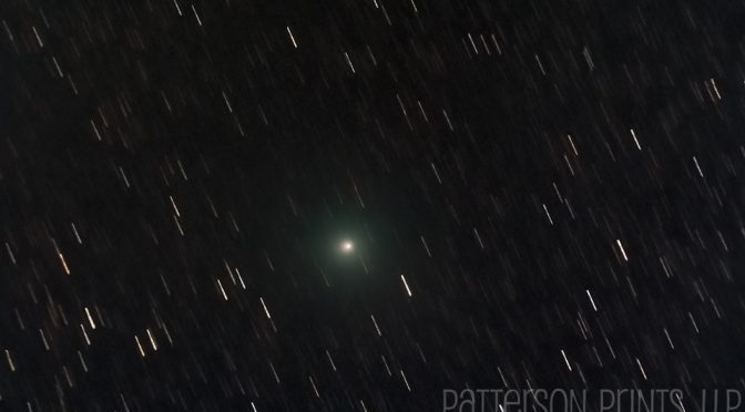
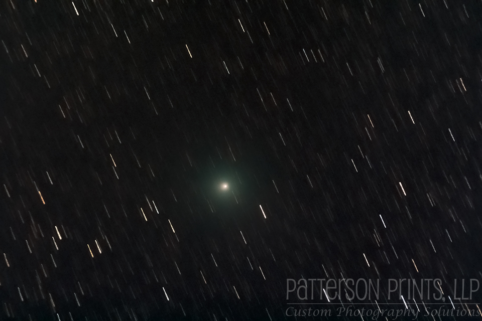
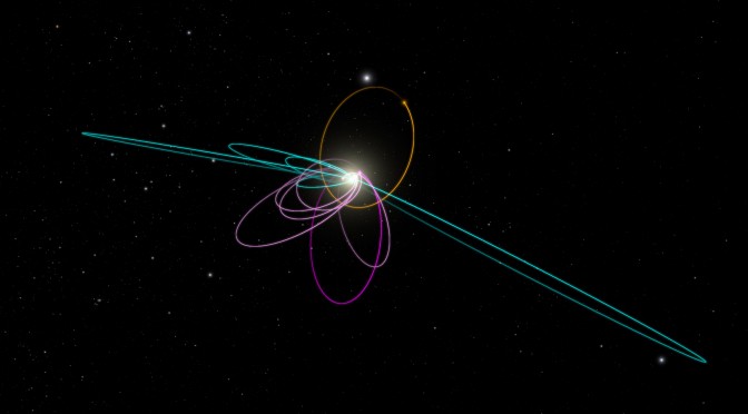
In January, right at the beginning of the Spring semester, Professor of Planetary Astronomy Michael Brown and Assistant Professor of Planetary Astronomy Konstantin Batygin, both from the California Institute of Technology, published a remarkable prediction in the Astronomical Journal, Evidence for a Distant Giant Planet in the Solar System (read the article here, http://web.gps.caltech.edu/~kbatygin/Publications_files/ms_planet9.pdf) In the article, Dr. Batygin, the theoretician of the pair, uses Dr. Brown’s observations of objects within the Kuiper Belt to argue for the existence of an object in a Sedna-like orbit and approximately ten times the mass of Earth. The basis for their claim is the ordered clustering of the perihelions of the orbits of multiple Kuiper Belt objects, a phenomenon that has a 0.007% of occurring randomly (yes, the significance of the number was not lost on me). After a significant amount of modelling and numerical analysis, Dr. Batygin predicts the likely orbital parameters of the Neptune-sized object as being inclined as much as 40 degrees to the ecliptic and having a semi-major axis of ~700 AU with an eccentricity of ~0.6. Kuiper_oort This places its perihelion around 280 AU. That’s really far out there, and places the proposed object as a member of the distant Kuiper Belt or inner Oort Cloud, or Hills Cloud, rather than a member of the inner Kuiper Belt wherein resides more familiar objects like Pluto and Eris. The mathematics are extremely compelling and the discussion and conclusions well-reasoned, but as the modern saying goes, “Pics or it didn’t happen.”

This certainly isn’t the first time that an object has been predicted to exist by mathematical analysis of the orbit of other objects. The most famous, and earliest, is the prediction by French astronomer and mathematician Urbain Le Verrier of the existence of an eighth planet beyond the orbit of Uranus that would account for the Uranus’ increase and subsequent decrease in orbital speed unrelated to its solar distance. Le Verrier worked on the problem in the summer of 1846 during his position at the Paris Observatory. Using Newton’s mechanics and Law of Gravity and the observed positions of Uranus, he calculated where a more distant planet would have to be and how massive it would have to be to produce the observed deviations. After completing his work, two astronomers, Johann Gottfried Galle and Heinrich Louis d’Arrest at the Berlin University, began searching in the vicinity of Le Verrier’s predicted position for the new planet. Galle, looking through the telescope, called out positions and brightnesses of the visible objects to d’Arrest who compared the observations to previously recorded charts until Galle called out an object that was not on the chart. They had found the planet that would later come to be called Neptune within a single degree of Le Verrier’s calculations. It was a remarkable piece of work from both Le Verrier and from Galle and d’Arrest, and it was a triumph for Newtonian mechanics.

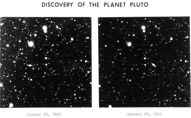
This method of discovering new objects was later attempted by William H. Pickering, Professor of Physics at Harvard University. Based on his calculations, using the apparent discrepancies in the orbits of both Uranus and Neptune, he attempted to image the proposed trans-Neptunian object at the Mount Wilson Observatory outside of Pasadena, CA. His search was unsuccessful, but the hunt for “Planet X” was picked up by Percival Lowell who had founded the Lowell Observatory in Flagstaff, AZ. Lowell’s attempts were equally unsuccessful. After Lowell’s passing, the search was tasked to an amateur astronomer from Burdett, KS, 23-year old Clyde Tombaugh. Rather than relying on sophisticated calculations, Tombaugh was tasked with systematically searching the Zodiac for anything non-stellar. In late January 1930, he captured two images of the object that we now know as Pluto. As it turns out the position of Pluto did not in any way correlate to Pickering’s calculations. In this case, the discrepancies were due to the lack of precision in the measurement of the masses of the outer planets.

discovery_of_Pluto_photographic_plate_comparison

Today, modern astronomers use the periodic motion of stars to mathematically infer the presence of extrasolar planets. The first of these discoveries was 51 Pegasi b. As two bodies orbit each other, such as a planet around its host star, the two bodies both move about their common center of mass. The planet being significantly less massive moves far more noticeably than the star, but the star does still move. Its motion is detectable by analysis of its light spectrum’s becoming alternately slightly bluer and then slightly redder as the star moves towards us and then away from us, respectively. This method has been used to locate many such extrasolar planets that we’re still unable to image directly. These are generally accepted as exceptions to the “Pics or it doesn’t exist” rule in science. The mathematics and analysis are so strongly compelling and there is no other viable alternate explanation that it is accepted that orbiting planetary bodies are responsible for the variations in the radial velocity of 51 Peg and other stars.

So now if we’re willing to take the mathematical word of the existence of extrasolar planets such as 51 Peg b, then why not for this new object proposed by Dr. Batygin and Dr. Brown from Cal Tech? The difference lies in the complexity of the problem. The extra solar planet problem is by comparison a simple problem. The radial velocity curve for 51 Peg is very clean, and the analysis of the data use methods that have long been vetted and refined by astronomers studying binary stars for which one can see the two separate objects. In other words, there is precedent for the methodology. This is not to say that Dr. Batygin’s methods are controversial or that the mathematical tools are not well understood. The Hamiltonian mechanics he deploys in his paper are extremely well understood and have been for over a century, but the data with which Dr. Batygin is working and the significant complexity created by moving from a two-body problem to an n-body problem make the analysis more difficult and intricate as well as making the results of those analyses less precise. For this reason, while I am very excited about this new prediction, I want to see an image before I take it as fact.

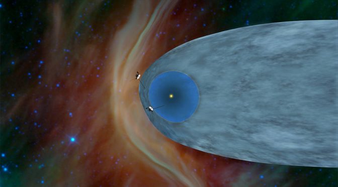
The observational discovery this new object, if it exists, likely won’t happen soon. Even at its proposed closest approach to the Sun, 280 AU, the intensity of sunlight striking the object is 0.00128% that of what it is here at Earth. Not only is the light very dim at that distance, most Kuiper Belt and inner Oort Cloud objects are coated with carbonaceous dust making their surfaces very dark and non-reflective. As our observational tools and techniques improve, we may eventually be able to start imaging these remote sentinels of our solar system, but until then, we’re left with only the predictions.

AGU14 – Day 1

If you jump in muddy puddles, you must wear your boots. Yeah, well, I don’t have boots. What I do have are two pairs of completely soaked socks, a pair of shoes that might dry out by March, and two very cold and tired feet! …I need wellies, or at least galoshes. It drizzled and rained all day long, which made getting from one building of the Moscone Center to another a bit of a miserable experience. Inside the sessions was quite a different matter, though.

There were several good talks about the behaviour of the magnetosphere and observations by the Van Allen Probes, but today the two most interesting talks I attended were about Mars. The first was about ancient lakes and outflows on the eastern portion of Valles Marineris. The presenter showed evidence on how the outflow from Eros Chaos was directed with estimations on the approximate time the area was drained based on the cratering density on the surface. By this time, it’s no surprise that there was abundant liquid water on the surface of Mars in the distant past, but it’s fun to see people starting to evaluate how that surface water flowed across the surface and how long it would have been present.

The other Mars talk I attended had the clickbait-style title, “How to snowboard on Mars”. What the talk was really about was providing an explanation of how numerous small gullies form on the sandy slopes of some ridge lines on Mars. At first glance, these gullies look remarkably like snowboard tracks. So… Aliens? No, dry ice. As the ice sublimates, the freshly formed vapour lifts the slab of ice off the surface slightly and serves as a lubricant allowing the slab to slide down the slope with enough energy to gouge out a furrow in the sandy surface. This phenomenon has been replicated with dry ice in the Mojave Desert. See the article on NASA’s website for more details.